Chapter 2 Initial Score Card

• Dropping Division, Nationality, Age, and Number of Children for regulatory requirements

accepts<-subset(accepts, select=-c(DIV, CHILDREN, NAT,  AGE))
rejects<-subset(rejects, select=-c(DIV, CHILDREN, NAT,  AGE))
accepts$good <- abs(accepts$GB - 1)

2.1 Exploratory Data Analysis

• unique value for each variable

print(as.data.frame(lapply(lapply(accepts,unique),length)))

##   PERS_H TMADD TMJOB1 TEL NMBLOAN FINLOAN INCOME EC_CARD BUREAU LOCATION LOANS REGN CASH PRODUCT RESID
## 1     10    32     33   3       3       2     27       2      3        2     9    9   29       7     3
##   PROF CAR CARDS GB X_freq_ good
## 1   10   3     7  2       2    2

set.seed(12345)
train_id <- sample(seq_len(nrow(accepts)), size = floor(0.70*nrow(accepts)))
train <- accepts[train_id, ]
test <- accepts[-train_id, ]

• Variable Classification
  • Categorical Variable
    1. Variable Level < = 10
    2. Variable Type is Character
  • Continuous Variables Not Continuous

col_unique<-lapply(lapply(train,unique),length)
catag_variable<-names(col_unique[col_unique<=10])
chara_type<-lapply(train,typeof)
chara_names<-names(chara_type[chara_type=="character"])
catag_variable<-unique(c(chara_names,catag_variable))
catag_variable<-subset(catag_variable,!(catag_variable%in%c("good")))
conti_variable<-names(train)
conti_variable<-subset(conti_variable,!(conti_variable%in%catag_variable))

Factorize the categorical variables

train[,catag_variable]=lapply(train[,catag_variable],as.factor)
test[,catag_variable]=lapply(test[,catag_variable],as.factor)

2.2 Variables Selection

• key_variable
  • Continuous Variables: Tenure, Income
  • Categorical Variables: Person in the household, Card Name, EC Card Holder

result_con <- list() # Creating empty list to store all results #
for(i in 1:length(conti_variable)){
  result_con[[conti_variable[i]]] <- smbinning(df = train, y = "good", x = conti_variable[i])
}

smbinning.sumiv.plot(iv_summary)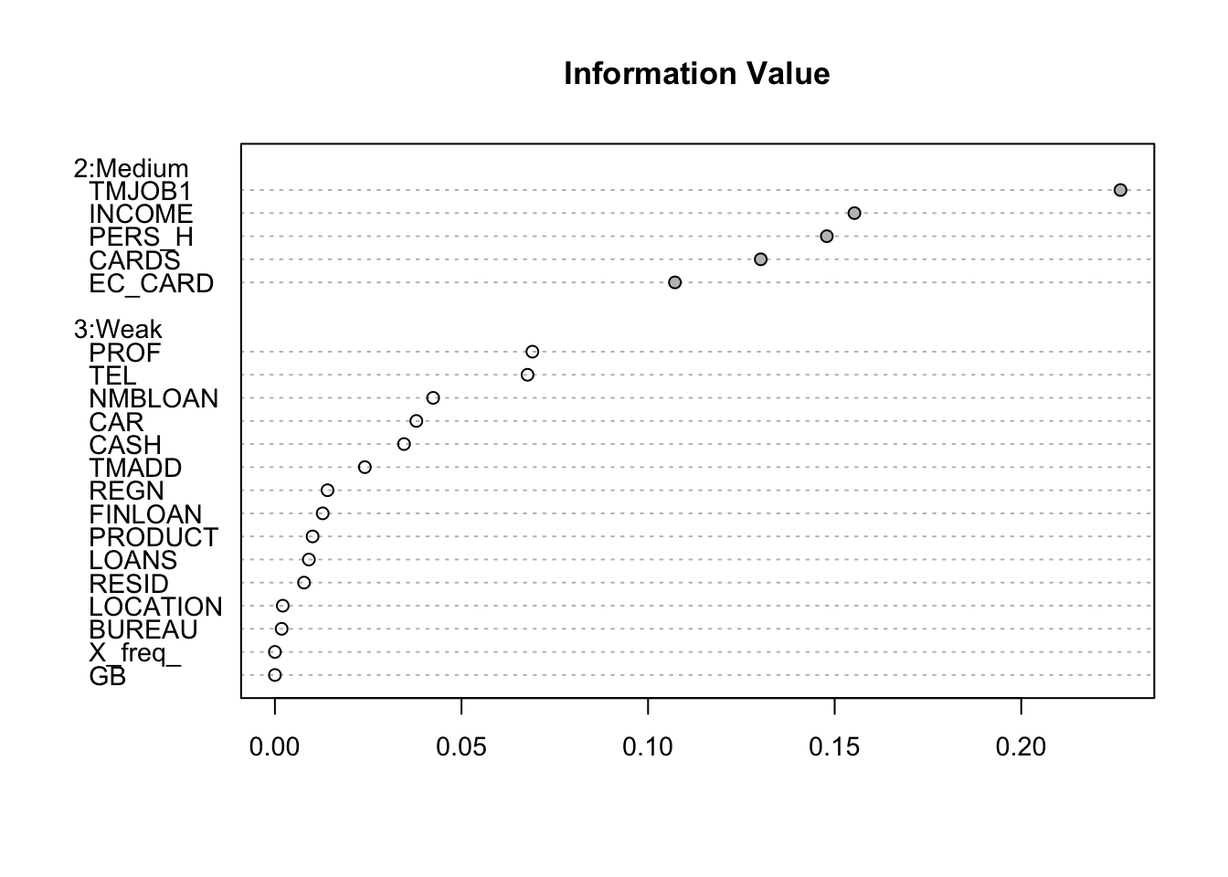

key_variable<-iv_summary$Char[iv_summary$IV>=0.1&is.na(iv_summary$IV)==FALSE]
results<-c(result_con)
result_all_sig<-results[key_variable]

2.3 Standardize Continuous Variables

• Bin continuous variables and Caclulate the WOE
• Add the Binned Variable and WOE to the original training dataset

for(i in 1:2) {
  train <- smbinning.gen(df = train, ivout = result_all_sig[[i]], chrname = paste(result_all_sig[[i]]$x, "_bin", sep = ""))
}

for (j in 1:2) {
  for (i in 1:nrow(train)) {
    bin_name <- paste(result_all_sig[[j]]$x, "_bin", sep = "")
    bin <- substr(train[[bin_name]][i], 2, 2)
    
    woe_name <- paste(result_all_sig[[j]]$x, "_WOE", sep = "")
    
    if(bin == 0) {
      bin <- dim(result_all_sig[[j]]$ivtable)[1] - 1
      train[[woe_name]][i] <- result_all_sig[[j]]$ivtable[bin, "WoE"]
    } else {
      train[[woe_name]][i] <- result_all_sig[[j]]$ivtable[bin, "WoE"]
    }
  }
}

2.4 Standardize Categorical Variables

• Calculate the WOE using the klaR package
• Add WOE to the original training dataset

train$good<-as.factor(train$good)
woemodel <- woe(good~., data = train, zeroadj=0.005, applyontrain = TRUE)

## At least one empty cell (class x level) does exists. Zero adjustment applied!
## At least one empty cell (class x level) does exists. Zero adjustment applied!
## At least one empty cell (class x level) does exists. Zero adjustment applied!
## At least one empty cell (class x level) does exists. Zero adjustment applied!
## At least one empty cell (class x level) does exists. Zero adjustment applied!
## At least one empty cell (class x level) does exists. Zero adjustment applied!
## At least one empty cell (class x level) does exists. Zero adjustment applied!
## At least one empty cell (class x level) does exists. Zero adjustment applied!
## At least one empty cell (class x level) does exists. Zero adjustment applied!

traindata <- predict(woemodel, train, replace = TRUE)

## No woe model for variable(s): good

train=cbind(train,traindata[,c("woe_CARDS","woe_PERS_H","woe_EC_CARD")])

############################## mapping tables for the categorical woe ##############################
cate1=unique(train[,c("CARDS","woe_CARDS")])
cate2=unique(train[,c("PERS_H","woe_PERS_H")])
cate3=unique(train[,c("EC_CARD","woe_EC_CARD")])
####################################################################################################

2.5 Initial Logistic Regression Model and Model Selection

train$X_freq_=as.numeric(as.character(train$X_freq_))
initial_score <- glm(data = train, GB ~  
                       TMJOB1_WOE + 
                       INCOME_WOE + woe_CARDS+woe_PERS_H+woe_EC_CARD
                     , weights =X_freq_,family = "binomial")

summary(initial_score)

## 
## Call:
## glm(formula = GB ~ TMJOB1_WOE + INCOME_WOE + woe_CARDS + woe_PERS_H + 
##     woe_EC_CARD, family = "binomial", data = train, weights = X_freq_)
## 
## Deviance Residuals: 
##     Min       1Q   Median       3Q      Max  
## -2.4537  -1.3243  -0.1546   2.5085   3.2984  
## 
## Coefficients:
##             Estimate Std. Error  z value             Pr(>|z|)    
## (Intercept) -3.40252    0.03328 -102.231 < 0.0000000000000002 ***
## TMJOB1_WOE  -0.86482    0.07856  -11.009 < 0.0000000000000002 ***
## INCOME_WOE  -0.17260    0.11370   -1.518                0.129    
## woe_CARDS    0.98698    0.24951    3.956            0.0000763 ***
## woe_PERS_H   0.82881    0.08009   10.348 < 0.0000000000000002 ***
## woe_EC_CARD -0.11756    0.27155   -0.433                0.665    
## ---
## Signif. codes:  0 '***' 0.001 '**' 0.01 '*' 0.05 '.' 0.1 ' ' 1
## 
## (Dispersion parameter for binomial family taken to be 1)
## 
##     Null deviance: 9272.2  on 2099  degrees of freedom
## Residual deviance: 8812.9  on 2094  degrees of freedom
## AIC: 8824.9
## 
## Number of Fisher Scoring iterations: 5

# Variable Selected Logistic Regression
initial_score_red <- glm(data = train, GB ~  
                           TMJOB1_WOE + 
                           woe_CARDS+woe_PERS_H
                         , weights =X_freq_,family = "binomial")

summary(initial_score_red)

## 
## Call:
## glm(formula = GB ~ TMJOB1_WOE + woe_CARDS + woe_PERS_H, family = "binomial", 
##     data = train, weights = X_freq_)
## 
## Deviance Residuals: 
##    Min      1Q  Median      3Q     Max  
## -2.434  -1.359  -0.150   2.495   3.279  
## 
## Coefficients:
##             Estimate Std. Error z value            Pr(>|z|)    
## (Intercept) -3.40238    0.03328 -102.25 <0.0000000000000002 ***
## TMJOB1_WOE  -0.88852    0.07713  -11.52 <0.0000000000000002 ***
## woe_CARDS    1.01760    0.09591   10.61 <0.0000000000000002 ***
## woe_PERS_H   0.84999    0.07905   10.75 <0.0000000000000002 ***
## ---
## Signif. codes:  0 '***' 0.001 '**' 0.01 '*' 0.05 '.' 0.1 ' ' 1
## 
## (Dispersion parameter for binomial family taken to be 1)
## 
##     Null deviance: 9272.2  on 2099  degrees of freedom
## Residual deviance: 8815.2  on 2096  degrees of freedom
## AIC: 8823.2
## 
## Number of Fisher Scoring iterations: 5

2.6 Evaluate the Initial Model - Training Data

## where predictions have outliers train$pred>=0.2
train$pred=predict(initial_score_red,data=train,type = "response")
train$GB<-as.numeric(as.character(train$GB))
train$good<-as.numeric(as.character(train$good))
smbinning.metrics(dataset = train, prediction = "pred", actualclass = "GB", report = 1)

## 
##   Overall Performance Metrics 
##   -------------------------------------------------- 
##                     KS : 0.2686 (Unpredictive)
##                    AUC : 0.6847 (Poor)
## 
##   Classification Matrix 
##   -------------------------------------------------- 
##            Cutoff (>=) : 0.0335 (Optimal)
##    True Positives (TP) : 704
##   False Positives (FP) : 423
##   False Negatives (FN) : 345
##    True Negatives (TN) : 628
##    Total Positives (P) : 1049
##    Total Negatives (N) : 1051
## 
##   Business/Performance Metrics 
##   -------------------------------------------------- 
##       %Records>=Cutoff : 0.5367
##              Good Rate : 0.6247 (Vs 0.4995 Overall)
##               Bad Rate : 0.3753 (Vs 0.5005 Overall)
##         Accuracy (ACC) : 0.6343
##      Sensitivity (TPR) : 0.6711
##  False Neg. Rate (FNR) : 0.3289
##  False Pos. Rate (FPR) : 0.4025
##      Specificity (TNR) : 0.5975
##        Precision (PPV) : 0.6247
##   False Discovery Rate : 0.3753
##     False Omision Rate : 0.3546
##   Inv. Precision (NPV) : 0.6454
## 
##   Note: 0 rows deleted due to missing data.

smbinning.metrics(dataset = train[train$pred<=0.2,], prediction = "pred", actualclass = "GB", report = 0, plot = "ks")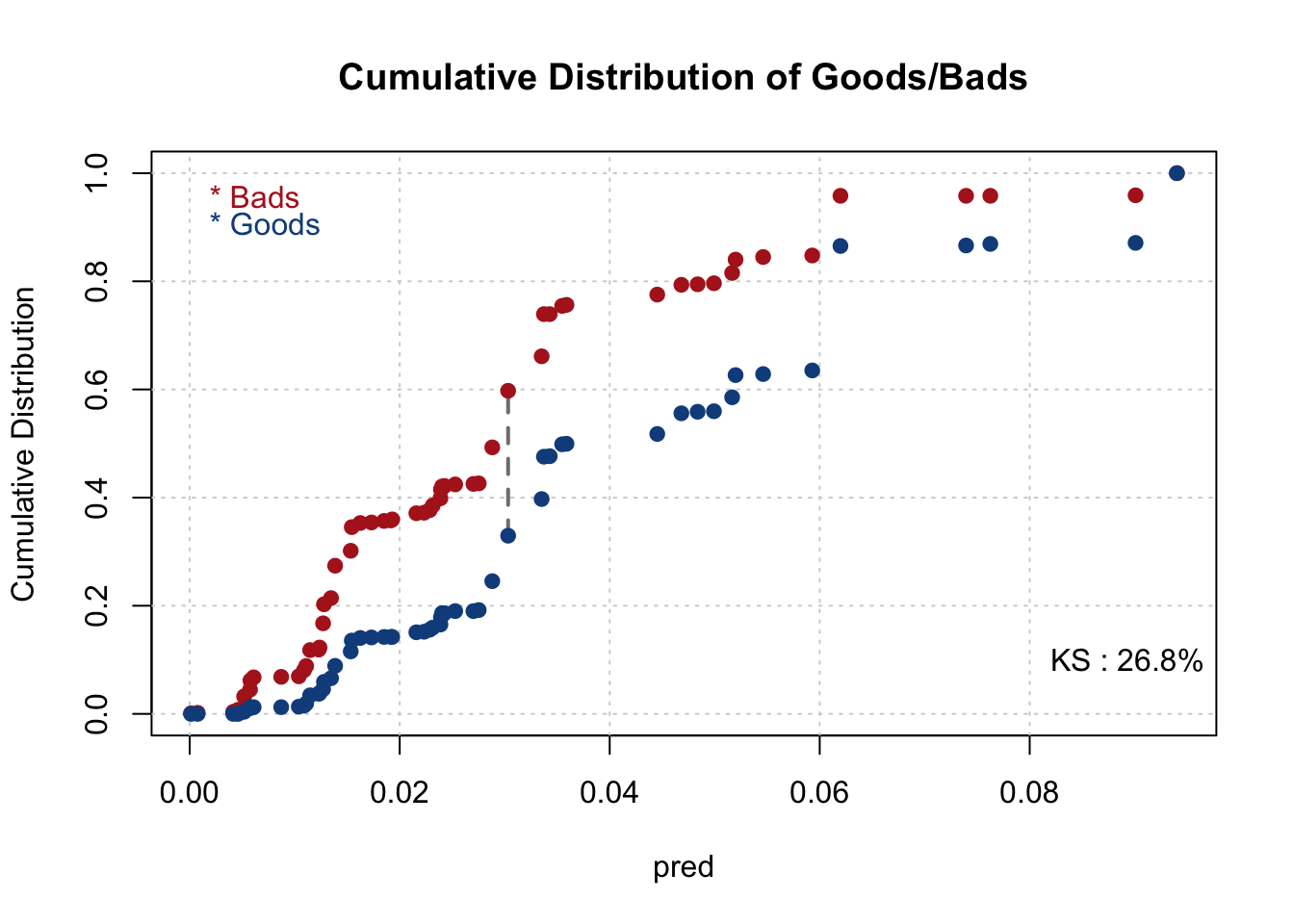

smbinning.metrics(dataset = train, prediction = "pred", actualclass = "GB", report = 0, plot = "auc")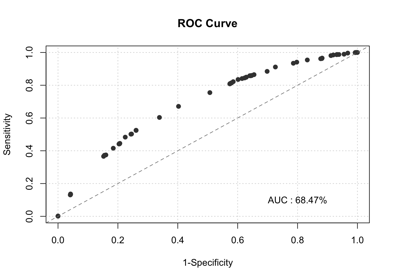

pred<-prediction(fitted(initial_score_red),factor(train$GB))
perf<-performance(pred,measure="tpr",x.measure="fpr")
plot(perf,lwd=3,colorsize=TRUE,colorkey=TRUE,colorsize.palette=rev(gray.colors(256)))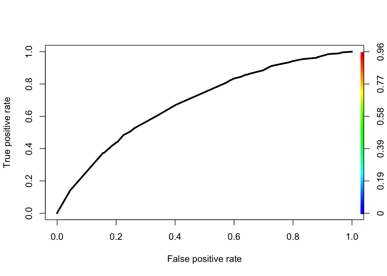

KS<-max(perf@y.values[[1]]-perf@x.values[[1]]) ## 0.03351922
cutoffAtKS<-unlist(perf@alpha.values)[which.max(perf@y.values[[1]]-perf@x.values[[1]])]
print(c(KS,cutoffAtKS))

## [1] 0.26864151 0.03351922

2.7 Evaluate the Initial Model - Testing Data

for(i in 1:2) {
  test <- smbinning.gen(df = test, ivout = result_all_sig[[i]], chrname = paste(result_all_sig[[i]]$x, "_bin", sep = ""))
}

for (j in 1:2) {
  for (i in 1:nrow(test)) {
    bin_name <- paste(result_all_sig[[j]]$x, "_bin", sep = "")
    bin <- substr(test[[bin_name]][i], 2, 2)
    
    woe_name <- paste(result_all_sig[[j]]$x, "_WOE", sep = "")
    
    if(bin == 0) {
      bin <- dim(result_all_sig[[j]]$ivtable)[1] - 1
      test[[woe_name]][i] <- result_all_sig[[j]]$ivtable[bin, "WoE"]
    } else {
      test[[woe_name]][i] <- result_all_sig[[j]]$ivtable[bin, "WoE"]
    }
  }
}

test$good<-as.factor(test$good)

########## categorical ####################################
test<-merge(test,cate1,by="CARDS",all.x = TRUE)
test<-merge(test,cate2,by="PERS_H",all.x = TRUE)
########## categorical ####################################

test$good=as.numeric(as.character(test$good))
test$GB=as.numeric(as.character(test$GB))
test$X_freq_=as.numeric(as.character(test$X_freq_))
test$pred <- predict(initial_score_red, newdata=test, type='response')
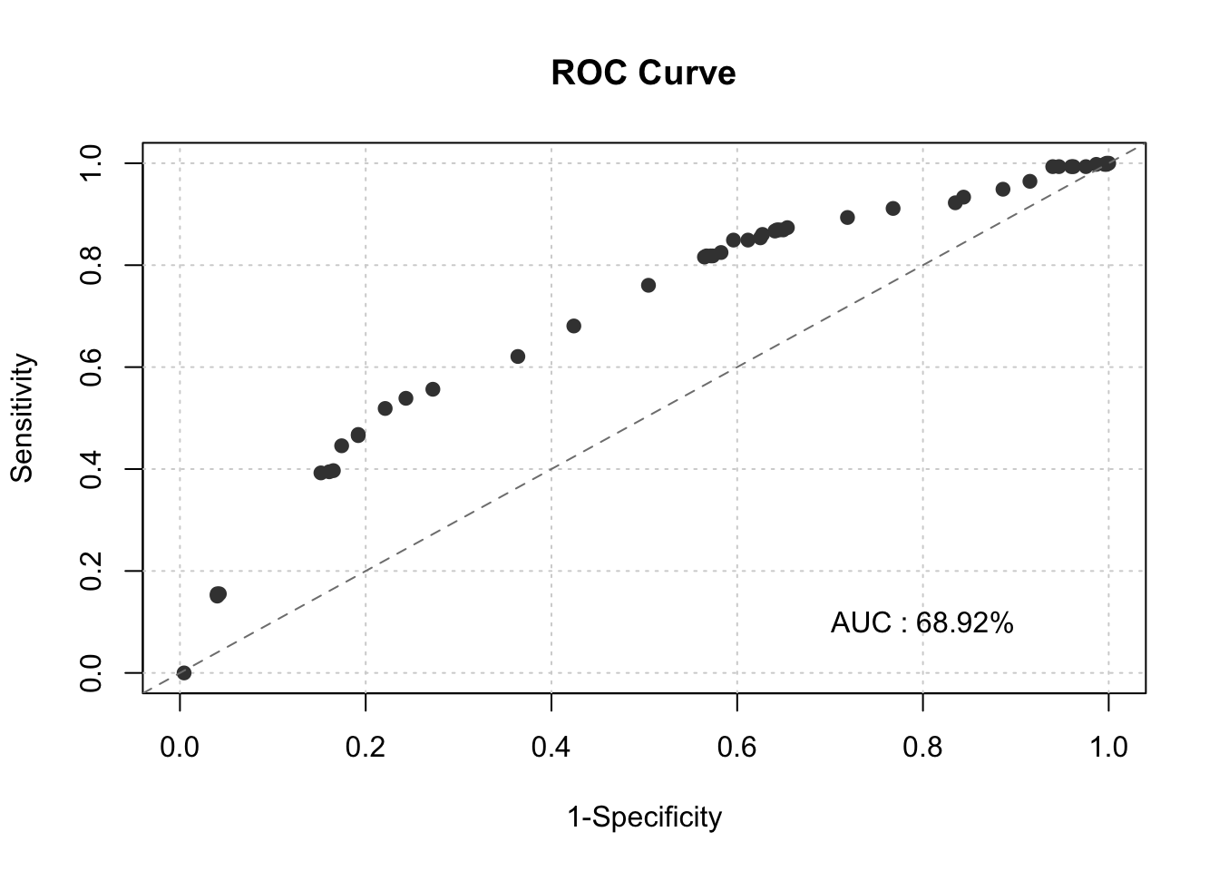
smbinning.metrics(dataset = test, prediction = "pred", actualclass = "GB", report = 1)

## 
##   Overall Performance Metrics 
##   -------------------------------------------------- 
##                     KS : 0.2979 (Unpredictive)
##                    AUC : 0.6892 (Poor)
## 
##   Classification Matrix 
##   -------------------------------------------------- 
##            Cutoff (>=) : 0.0468 (Optimal)
##    True Positives (TP) : 234
##   False Positives (FP) : 99
##   False Negatives (FN) : 217
##    True Negatives (TN) : 349
##    Total Positives (P) : 451
##    Total Negatives (N) : 448
## 
##   Business/Performance Metrics 
##   -------------------------------------------------- 
##       %Records>=Cutoff : 0.3704
##              Good Rate : 0.7027 (Vs 0.5017 Overall)
##               Bad Rate : 0.2973 (Vs 0.4983 Overall)
##         Accuracy (ACC) : 0.6485
##      Sensitivity (TPR) : 0.5188
##  False Neg. Rate (FNR) : 0.4812
##  False Pos. Rate (FPR) : 0.2210
##      Specificity (TNR) : 0.7790
##        Precision (PPV) : 0.7027
##   False Discovery Rate : 0.2973
##     False Omision Rate : 0.3834
##   Inv. Precision (NPV) : 0.6166
## 
##   Note: 1 rows deleted due to missing data.

smbinning.metrics(dataset = test[test$pred<=0.2,], prediction = "pred", actualclass = "GB", report = 0, plot = "ks")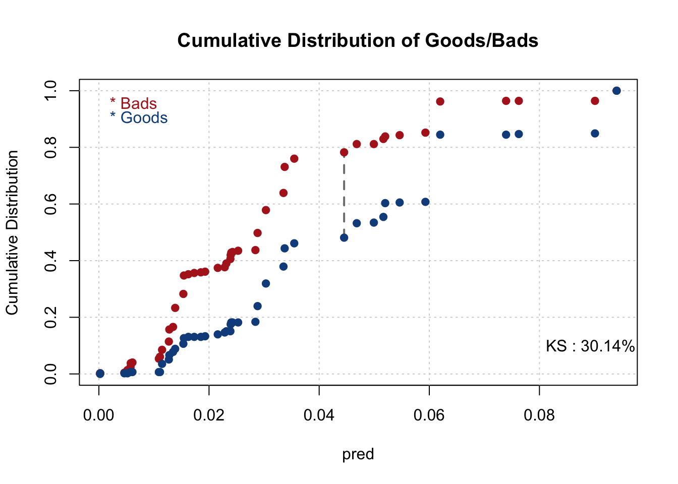

smbinning.metrics(dataset = test, prediction = "pred", actualclass = "GB", report = 0, plot = "auc")